Large Language Models in the Social Sciences

DAY FIVE GESIS Fall Seminar in Computational Social Science

Johannes B. Gruber

GESIS

Introduction

Schedule: GESIS Fall Seminar in Computational Social Science

Course Schedule
time Session
Day 1 Introduction to Computational Social Science
Day 2 Obtaining Data
Day 4 Computational Network Analysis
Day 4 Computational Text Analysis
Day 5 Large Language Models in the Social Sciences

The Plan for Today

  • Overview: what are LLMs (are they artificial intelligence?)
  • How we can use them for Computational Social Science Research
  • How can we use them for Computational Text Analysis

Maximalfocus via unsplash.com

What are Large Language Models?

What are language models?

Language models are statistical representations of natural language that use machine learning to model relationships between words

Examples:

  • Supervised Machine Learning Models: text input → category output
  • Unsupervised Machine Learning Models: relationship between words and words; words and texts; texts and texts
  • Machine Translation Models: input text → output text
  • Generative Language Models: fill in blanks in a sentence

Timeline language models

Source: Computational Analysis of Digital Communication

Timeline language models

Source: Computational Analysis of Digital Communication

The initial problem of text analysis

  • Computers don’t read text, they only can deal with numbers

  • For this reason, so far, we tokenized our texts (e.g., in words) and summarized their frequency across texts to create a document-feature matrix within the bag-of-words model

  • Such a text representation has some issues:

    • Treats words as equally important (→ requires removal of noise, stopwords…)
    • Ignores word order and context
    • Results in a sparse matrix (→ computationally expensive)

Alternative: Map words into a vector space

What are embeddings?

  • featuere-topic-matrix

This case makes it pretty clear:

  • mice belong into the first topic
  • cats belong into the second
  • dogs belong into the third topic

Pre-trained Word embeddings: GloVe

library(tidyverse)
get_glove <- function(dir, dimensions = c(50, 100, 200, 300)) {
  # don't re-download files if present
  file <- file.path(dir, paste0("glove.6B.", dimensions, "d.txt"))
  cache_loc <- file.path(dir, "glove.6B.zip")
  if (!file.exists(file)) {    
    if (!file.exists(cache_loc)) {
      curl::curl_download("http://nlp.stanford.edu/data/glove.6B.zip", cache_loc, quiet = FALSE)
    }
    unzip(cache_loc, files = basename(file), exdir = "data")
  }
  # read and process glove vectors
  df <- data.table::fread(file, quote = "")
  colnames(df) <- c("term", paste0("dim", seq_len(ncol(df) - 1)))
  return(df)
}
glove_df <- get_glove("data", dimensions = 50)

# 10 highest scoring words on dimension 1
glove_df |> 
  arrange(-dim1) |> 
  select(1:10)
                   term    dim1     dim2      dim3      dim4      dim5
                 <char>   <num>    <num>     <num>     <num>     <num>
     1:  tenebrionoidea  3.8740 -1.55920  0.473120 -0.013167  1.125800
     2:           ncrna  3.3151  0.60170  0.055274 -0.465000  0.359460
     3:      polychaete  3.2700 -1.88100  0.038965 -0.166440  0.851370
     4:          power8  3.2423 -1.27580 -0.212460 -0.836850 -1.374200
     5:     mordellidae  3.2301  0.29574 -2.045200  0.444990 -0.036238
    ---                                                               
399996:      boys/girls -3.9372  0.81523  0.552410  0.881190 -0.644110
399997:             fbh -4.0441  1.72390 -0.474970 -1.766100 -1.229500
399998: a-international -4.1408  1.28900 -1.648300 -1.939000 -0.212160
399999:      music/club -4.4444  0.12984 -1.458600  0.930280 -1.027600
400000:           20003 -5.4593  0.89405 -0.297340  2.285400  0.022355
             dim6     dim7     dim8      dim9
            <num>    <num>    <num>     <num>
     1: -0.109480  0.21668  1.95260  1.480300
     2:  0.585580  1.29810 -0.79698  0.724100
     3: -0.545460  0.75165 -1.37070 -0.239080
     4:  0.146710  0.47105 -0.78261 -0.387710
     5: -0.666850 -1.22810  0.19445  1.300100
    ---                                      
399996: -2.449200  0.45895 -0.68265  1.352400
399997: -0.874810 -0.82598 -0.89391  0.080878
399998:  0.026836  0.50593  1.58940 -0.223550
399999: -0.525320  0.99353  0.67030  0.429440
400000: -1.597400 -1.16780 -1.90480  0.027555

Similarities between words

As mentioned before, we can compute similarity scores for word pairs:

nearest_neighbors <- function(tbl, word, n = 15) {
  
  comp <- filter(tbl, term == word)
  if (nrow(comp) < 1L) stop("word ", word, " not found in the embedding")
  sim <- proxyC::simil(as.matrix(select(comp, -term)), 
                       as.matrix(select(tbl, -term)), 
                       method = "cosine") # calculate cosine similarity
  # get the n highest values plus original word
  rank <- order(as.numeric(sim), decreasing = TRUE)[seq_len(n + 1)] 
  tibble(
    word = word,
    neighbor = tbl$term[rank],
    similarity = sim[1, rank]
  )
}
nearest_neighbors(glove_df, "basketball")
# A tibble: 16 × 3
   word       neighbor     similarity
   <chr>      <chr>             <dbl>
 1 basketball basketball        1    
 2 basketball football          0.879
 3 basketball hockey            0.862
 4 basketball baseball          0.861
 5 basketball nba               0.838
 6 basketball soccer            0.820
 7 basketball athletics         0.805
 8 basketball softball          0.800
 9 basketball junior            0.799
10 basketball coaching          0.797
11 basketball coached           0.792
12 basketball team              0.789
13 basketball varsity           0.779
14 basketball ncaa              0.771
15 basketball championship      0.770
16 basketball volleyball        0.768
nearest_neighbors(glove_df, "netherlands")
# A tibble: 16 × 3
   word        neighbor    similarity
   <chr>       <chr>            <dbl>
 1 netherlands netherlands      1    
 2 netherlands belgium          0.893
 3 netherlands switzerland      0.821
 4 netherlands denmark          0.809
 5 netherlands france           0.789
 6 netherlands sweden           0.787
 7 netherlands dutch            0.782
 8 netherlands germany          0.772
 9 netherlands austria          0.764
10 netherlands luxembourg       0.716
11 netherlands holland          0.716
12 netherlands spain            0.708
13 netherlands britain          0.701
14 netherlands canada           0.700
15 netherlands amsterdam        0.698
16 netherlands italy            0.693

Similarity of entire sentences or texts

But we can also generalize word embeddings to entire sentences (or even texts):

library(rollama)

# Example sentences
movies <- tibble(sentences = c("This movie is great, I loved it.", 
                               "The film was fantastic, a real treat!",
                               "I did not like this movie, it was not great.",
                               "Today, I went to the cinema and watched a movie",
                               "I had pizza for lunch."))
                     
# Get embeddings from a sentence transformer
movie_embeddings <- embed_text(movies$sentences, model = "nomic-embed-text")

# Each text has now 768 values
movie_embeddings 
# A tibble: 5 × 768
     dim_1   dim_2 dim_3    dim_4  dim_5  dim_6  dim_7 dim_8  dim_9  dim_10 dim_11 dim_12 dim_13 dim_14 dim_15 dim_16
     <dbl>   <dbl> <dbl>    <dbl>  <dbl>  <dbl>  <dbl> <dbl>  <dbl>   <dbl>  <dbl>  <dbl>  <dbl>  <dbl>  <dbl>  <dbl>
1 -0.00513  0.311  -3.61  0.220    0.113 0.702  -0.512 0.722 -0.170  0.276   0.218   1.90  0.867  0.265  0.290  -1.41
2  0.495    0.999  -4.24  0.0294  -0.782 0.490  -0.662 1.73   0.115 -0.0209  0.343   1.96  1.62   0.838  0.671  -1.36
3 -0.136    0.366  -2.53 -0.00299 -0.898 2.38   -0.138 0.594 -0.251  0.0802 -0.377   2.30  1.04   0.483 -0.260  -1.54
4 -0.877   -0.0846 -3.03 -0.672    0.740 0.649   0.240 0.803 -0.433 -0.459  -0.403   1.81  1.30   0.769  0.342  -1.87
5  1.73     1.22   -3.22  0.153    0.168 0.0506 -1.05  0.911 -0.789 -0.907  -0.583   1.38  0.558  0.567 -0.548  -1.50
# ℹ 752 more variables: dim_17 <dbl>, dim_18 <dbl>, dim_19 <dbl>, dim_20 <dbl>, dim_21 <dbl>, dim_22 <dbl>,
#   dim_23 <dbl>, dim_24 <dbl>, dim_25 <dbl>, dim_26 <dbl>, dim_27 <dbl>, dim_28 <dbl>, dim_29 <dbl>, dim_30 <dbl>,
#   dim_31 <dbl>, dim_32 <dbl>, dim_33 <dbl>, dim_34 <dbl>, dim_35 <dbl>, dim_36 <dbl>, dim_37 <dbl>, dim_38 <dbl>,
#   dim_39 <dbl>, dim_40 <dbl>, dim_41 <dbl>, dim_42 <dbl>, dim_43 <dbl>, dim_44 <dbl>, dim_45 <dbl>, dim_46 <dbl>,
#   dim_47 <dbl>, dim_48 <dbl>, dim_49 <dbl>, dim_50 <dbl>, dim_51 <dbl>, dim_52 <dbl>, dim_53 <dbl>, dim_54 <dbl>,
#   dim_55 <dbl>, dim_56 <dbl>, dim_57 <dbl>, dim_58 <dbl>, dim_59 <dbl>, dim_60 <dbl>, dim_61 <dbl>, dim_62 <dbl>,
#   dim_63 <dbl>, dim_64 <dbl>, dim_65 <dbl>, dim_66 <dbl>, dim_67 <dbl>, dim_68 <dbl>, dim_69 <dbl>, dim_70 <dbl>, …

The subtle similarity of some texts in the example

  • We can see that text 2 is most similar to text 1: Both express a very similar sentiment, just with different words (“great” ≈ “fantastic”; “I loved it” ≈ “A real treat”)

  • Text 2 is still similar to text 3 (after all it is about movies), but less so compared to text 1 (“fantastic” is the opposite of “not great”)

  • Text 4 still shares similarities (the context is the cinema/watching movies), but text 5 is very different as it doesn’t contain similar words and is not about similar things (except “I”).

sim <- proxyC::simil(as.matrix(movie_embeddings), as.matrix(movie_embeddings), method = "cosine")
colnames(sim) <- paste0("movie", 1:5)
cbind(movies, as_tibble(as.matrix(sim)))
                                        sentences    movie1    movie2    movie3    movie4    movie5
1                This movie is great, I loved it. 1.0000000 0.7679983 0.7046627 0.6746315 0.4757985
2           The film was fantastic, a real treat! 0.7679983 1.0000000 0.6022398 0.6897439 0.4943511
3    I did not like this movie, it was not great. 0.7046627 0.6022398 1.0000000 0.6220552 0.4801814
4 Today, I went to the cinema and watched a movie 0.6746315 0.6897439 0.6220552 1.0000000 0.5786763
5                          I had pizza for lunch. 0.4757985 0.4943511 0.4801814 0.5786763 1.0000000

From Sparse to Dense Matrix Representation

  • Using embedding vectors instead of word frequencies further has the advantages of strongly reducing the dimensionality of the DTM: instead of (tens of) thousands of columns for each unique word we only need hundreds of columns for the embedding vectors (→ dense instead of sparse)

  • This means that further processing can be more efficient as fewer parameters need to be fit, or conversely that more complicated models can be used without blowing up the parameter space.

What are transformers?

  • Until 2017, the state-of-the-art for natural language processing was using a deep neural network (e.g., recurrent neural networks, long short-term memory and gated recurrent neural networks)
  • In a preprint called “Attention is all you need” (Vaswani et al. 2017), published in 2017 and cited more than 95,000 times, the team of Google Brain introduced the so-called Transformer, a a neural network-type architecture that learns context and thus meaning by tracking relationships in sequential data like the words in this sentence.
  • Transformer models apply an evolving set of mathematical techniques, called attention or self-attention, to detect subtle ways even distant data elements in a series influence and depend on each other.

Self-Attention

  • In general terms, self-attention works encodes how similar each word is to all the words in the sentence, including itself.

  • Once the similarities are calculated, they are used to determine how the transformers encodes each word.

Self-Attention

  • In general terms, self-attention works encodes how similar each word is to all the words in the sentence, including itself.

  • Once the similarities are calculated, they are used to determine how the transformers encodes each word.

Self-Attention

  • In general terms, self-attention works encodes how similar each word is to all the words in the sentence, including itself.

  • Once the similarities are calculated, they are used to determine how the transformers encodes each word.

Self-Attention

  • In general terms, self-attention works encodes how similar each word is to all the words in the sentence, including itself.

  • Once the similarities are calculated, they are used to determine how the transformers encodes each word.

So why are transformer models important?

  • Transformer models apply an evolving set of mathematical techniques, called attention or self-attention, to detect subtle ways even distant data elements in a series influence and depend on each other.
  • this actually simplifies learning:
    • No need for recurrent or convolutional network structures
    • Based solely on attention mechanism (stacked on top of one another)
    • Required less training time (can be parallelized)
  • It thereby outperformed prior state-of-the-art models in a variety of tasks
  • The transformer architecture is the back-bone of all current large language models and so far drives the entire “AI revolution”

Source: Vaswani et al. (2017)

Source: Vaswani et al. (2017)

What are Large language models

  • Large language models are language models that are large
  • Like the “big” in “big” data, the term is relative to what is considered at the time
  • It refers to the training data, the parameter size, and the computational resources needed for training
  • As models get larger, they approach what appears like general-purpose language understanding
  • Current generations of LLMs are still just a type of artificial neural networks (mainly transformers!) and are (pre-)trained using self-supervised learning and semi-supervised learning

What are generative large language models

  • trained to predict/generate next word in a conversation
  • surprisingly good at emulating humans to complete tasks
  • can be controlled with natural language
  • have become very popular through ChatGPT (a browser interface to communicate with OpenAI’s GPT models)

Next token prediction

Model categories

Technical things aside…

  • LLMs are probabilistic, not deterministic
  • LLMs are “stochastic parrots” mimicking human speech patterns observed in their training corpus (Bender et al. 2021)

Technical things aside…

  • LLMs are probabilistic, not deterministic
  • LLMs are “stochastic parrots” mimicking human speech patterns observed in their training corpus (Bender et al. 2021)
  • LLMs are trained to please and sound confident and eloquent
  • LLMs of “hallucinate” (or bullshit (Frankfurt 2005))

Hicks, Humphries, and Slater (2024)

Hicks, Humphries, and Slater (2024)

Technical things aside…

  • LLMs are probabilistic, not deterministic
  • LLMs are “stochastic parrots” mimicking human speech patterns observed in their training corpus (Bender et al. 2021)
  • LLMs are trained to please and sound confident and eloquent
  • LLMs of “hallucinate” (or bullshit (Frankfurt 2005))
  • “All quantitative models of language are wrong—but some are useful” (Grimmer and Stewart 2013)

Weber and Reichardt (2023)

Weber and Reichardt (2023)

How can we use LLMS for Computational Social Science Research

Some use cases

  • Survey Research: Automated coding and response generation
  • Experimental Studies: Creating stimuli and analyzing responses
  • Hypothesis Generation: Theory development assistance
  • Interview Analysis: Qualitative data coding
  • Content Analysis: Processing large text datasets
  • Writing and editing
  • Literature review
  • Programming

Maximalfocus via unsplash.com

Example: Using ‘AI’ web scrapers

Essentially two kinds of ‘AI’ web scrapers:

‘AI’ parsers

  • download html of a website
  • prompt ‘AI’ to extract certain information and return in a good structure

advantages :

  • no scraping skills needed whatsoever
  • can deal with complicated structures

disadvantages :

  • expensive (computational, time, but also 💸)
  • does not scale well
  • limit on the length of html content (depends on model context)
  • potential for hallucination

verdict:

👉 don’t believe the hype, skip this one

Using ‘AI’ web scrapers

Essentially two kinds of ‘AI’ web scrapers:

‘AI’ written parsers

  • download html of a website
  • prompt ‘AI’ to extract appropriate CSS selectors / write R code

advantages :

  • only some scraping skills needed
  • can deal with complicated structures
  • scales well

disadvantages :

  • potential for hallucination (and inaccuracies)
  • limit on the length of html content (depends on model context)

verdict:

👉 try to use them (but with tests and caution!)

Using ‘AI’ web scrapers

Essentially two kinds of ‘AI’ web scrapers:

‘AI’ parsers

  • download html of a website
  • prompt ‘AI’ to extract certain information and return in a good structure

advantages :

  • no scraping skills needed whatsoever
  • can deal with complicated structures

disadvantages :

  • expensive (computational, time, but also 💸)
  • does not scale well
  • limit on the length of html content (depends on model context)
  • potential for hallucination

verdict:

👉 don’t believe the hype, skip this one

‘AI’ written parsers

  • download html of a website
  • prompt ‘AI’ to extract appropriate CSS selectors / write R code

advantages :

  • only some scraping skills needed
  • can deal with complicated structures
  • scales well

disadvantages :

  • potential for hallucination (and inaccuracies)
  • limit on the length of html content (depends on model context)

verdict:

👉 try to use them (but with tests and caution!)

Example: Using ‘AI’ for programming

Let ‘AI’ write your code (aka. vibe coding)

  • prompt ‘AI’ to write your application/analysis code for you

advantages :

  • no programming skills needed whatsoever to write the code
  • can produce software with some impressive features

disadvantages :

  • you need to understand programming logic to prompt effectivly
  • if something goes wrong, this is very hard to fix
  • you might not even realize many of the issue

verdict:

👉 don’t believe the hype, being able to read+write code is still an important skill

Let ‘AI’ help you write code

  • you know what code you need / what it needs to do and which language packages you want to use
  • you prompt ‘AI’ to write a first draft of the code for you

advantages :

  • only some programming skills needed to write the code
  • can speed up your programming
  • can help you with “busy work” (writing documentation and comments)

disadvantages :

  • instead of writing code, you spend most of your time reviewing and debugging code
  • difficult to know in advance when it will save or waste time

verdict:

👉 try to use them (but with tests and caution!)

How can we use them for Computational Text Analysis

Why use gLLMs?

  • cheaper to use 💸 (experts > research assistants > crowd workers > gLLMs)
  • more accurate 🧠 (experts > research assistants > gLLMs > crowd workers)
  • better at annotating complex categories 🤔 (human* > gLLM > LLM > SML)
  • can use contextual information (human* > gLLM > LLM > ❌ SML)
  • multilingual1
  • easier* to use: plain English prompting

(e.g., Gilardi, Alizadeh, and Kubli 2023; Heseltine and Hohenberg 2023; Zhong et al. 2023; Törnberg 2023)

How do you work with them - simple example

OpenAI GPT via API

library(askgpt)
options(askgpt_chat_model = "gpt-4")
askgpt("What are generative Large Language Models?")
#> ── Answer ────────────────────────────────────────────────────────
#> Generative Large Language Models are artificial
#> intelligence models that generate human-like text.
#> They are designed to understand and predict human 
#> language patterns. GPT-3 by OpenAI is a good 
#> example of a Generative Large Language Model. 
#> They can generate stories, poems, or even technical
#> content.
#>
#> These models are 'generative' because they create 
#> (or generate) new content. They are 'large' because
#> they are trained on large amounts of data, and the 
#> term 'language model' is due to their ability to 
#> use and understand human language. They learn to 
#> produce text by being fed huge amounts of existing 
#> text data, learning patterns and context from that 
#> data, and using this understanding to create new, 
#> relevant text that follows the rules of the 
#> language it was trained on. 

Running model locally through Ollama

library(rollama)
query("What are generative Large Language Models?", model = "llama3:8b")
#> ── Answer from llama3:8b───────────────────────────────────────────
#> 
#> Generative large language models (LLMs) are a type
#> of artificial intelligence (AI) model that is
#> capable of generating new, > original text or
#> language based on patterns and structures learned
#> from large datasets. These models have become
#> increasingly popular in recent years due to their
#> ability to generate human-like text, respond to
#> questions, and even create entire stories.
#> 
#> Here's how they work: 
#> 
#> 1. **Training**: Generative LLMs are trained on 
#> massive amounts of text data, which can be sourced
#> from various places like books, articles, social
#> media, or online forums. 
#> 2. **Language patterns**: The models analyze the training data to identify patterns,
#> relationships, and structures in language. This
#> helps them learn how to generate new text that is
#> coherent, natural-sounding, and meaningful.
#> 3. **Generator**: The trained model has a generator
#> component that produces new text based on the
#> learned patterns. This can be done by sampling
#> from probability distributions or using techniques
#> like autoregressive models.
#> 4. **Conditioning**: To control the output of the 
#> model, conditioning mechanisms are used to specify
#> what kind of text should be generated. For example,
#> you might provide a prompt or topic for the model
#> to generate text about. 
#> 
#> Some key characteristics of generative LLMs include:
#> 
#> 1. **Autoregressive**: Generative models predict 
#> the next token in a sequence (e.g., word) based on 
#> the previous tokens.
#> 2. **Probabilistic**: The models assign 
#> probabilities to each possible output, allowing 
#> them to generate diverse and creative text.
#> 3. **Adversarial training**: Some models are trained
#> using adversarial examples, which helps them learn
#> to generate text that is more realistic and
#> challenging for humans to distinguish from
#> human-written text. 
#> 
#> Applications of generative LLMs:
#> 
#> 1. **Text generation**: These models can
#> be used to generate text for various purposes, such
#> as chatbots, customer service > responses, or
#> content marketing.  
#> 2. **Language translation**:
#> Generative LLMs can be fine-tuned for language
#> translation tasks, allowing them to translate text
#> from one language to another.
#> 3. **Content
#> creation**: They can help generate new ideas,
#> stories, or scripts by providing a starting point
#> and then > continuing the narrative.
#> 4. **Summarization**: Generative models can summarize
#> long pieces of text into shorter summaries while
#> preserving the original meaning.
#> 
#> Some popular examples of generative LLMs include: 
#> 
#> 1. **OpenAI's GPT-3**: A highly advanced language 
#> model capable of generating human-like text and 
#> responding to questions. 
#> 2. **Google's BERT**: A transformer-based model 
#> that has achieved state-of-the-art results in 
#> various natural language processing (NLP) tasks, 
#> including sentiment analysis and question answering.
#> 
#> These models have the potential to revolutionize 
#> many areas, from customer service and content 
#> creation to creative writing and > education.
#> However, they also require careful consideration 
#> of their ethical implications and limitations.

Classification–Strategies

Prompting strategies
Prompting Strategy Example Structure
Zero-shot {"role": "system", "content": "Text of System Prompt"},
{"role": "user", "content": "(Text to classify) + classification question"}
One-shot {"role": "system", "content": "Text of System Prompt"},
{"role": "user", "content": "(Example text) + classification question"},
{"role": "assistant", "content": "Example classification"},
{"role": "user", "content": "(Text to classify) + classification question"}
Few-shot {"role": "system", "content": "Text of System Prompt"},
{"role": "user", "content": "(Example text) + classification question"},
{"role": "assistant", "content": "Example classification"},
{"role": "user", "content": "(Example text) + classification question"},
{"role": "assistant", "content": "Example classification"},
. . . more examples
{"role": "user", "content": "(Text to classify) + classification question"}
Chain-of-Thought {"role": "system", "content": "Text of System Prompt"},
{"role": "user", "content": "(Text to classify) + reasoning question"},
{"role": "assistant", "content": "Reasoning"},
{"role": "user", "content": "Classification question"}

See: Weber and Reichardt (2023)

Classification–Zero-shot

q <- tribble(
  ~role,    ~content,
  "system", "You assign texts into categories. Answer with just the correct category.",
  "user",   "text: the pizza tastes terrible\ncategories: positive, neutral, negative"
)
query(q)

Classification–One-shot

q <- tribble(
  ~role,    ~content,
  "system", "You assign texts into categories. Answer with just the correct category.",
  "user", "text: the pizza tastes terrible\ncategories: positive, neutral, negative",
  "assistant", "Category: Negative",
  "user", "text: the service is great\ncategories: positive, neutral, negative"
)
query(q)
#> 
#> ── Answer ────────────────────────────────────────────────────────
#> Category: Positive

Neat effect: change the output structure

q <- tribble(
  ~role,    ~content,
  "system", "You assign texts into categories. Answer with just the correct category.",
  "user", "text: the pizza tastes terrible\ncategories: positive, neutral, negative",
  "assistant", "{'Category':'Negative','Confidence':'100%','Important':'terrible'}",
  "user", "text: the service is great\ncategories: positive, neutral, negative"
)
answer <- query(q)
#> 
#> ── Answer ────────────────────────────────────────────────────────
#> {'Category':'Positive','Confidence':'100%','Important':'great'}

Classification–Few-shot

q <- tribble(
  ~role,    ~content,
  "system", "You assign texts into categories. Answer with just the correct category.",
  "user", "text: the pizza tastes terrible\ncategories: positive, neutral, negative",
  "assistant", "Category: Negative",
  "user", "text: the service is great\ncategories: positive, neutral, negative",
  "assistant", "Category: Positive",
  "user", "text: I once came here with my wife\ncategories: positive, neutral, negative",
  "assistant", "Category: Neutral",
  "user", "text: I once ate pizza\ncategories: positive, neutral, negative"
)
query(q)

Classification–Chain-of-Thought

q_thought <- tribble(
  ~role,    ~content,
  "system", "You assign texts into categories. ",
  "user",   "text: the pizza tastes terrible\nWhat sentiment (positive, neutral, or negative) would you assign? Provide some thoughts."
)
output_thought <- query(q_thought)

Now we can use these thoughts in classification

q <- tribble(
  ~role,    ~content,
  "system", "You assign texts into categories. ",
  "user",   "text: the pizza tastes terrible\nWhat sentiment (positive, neutral, or negative) would you assign? Provide some thoughts.",
  "assistant", pluck(output_thought, "message", "content"),
  "user",   "Now answer with just the correct category (positive, neutral, or negative)"
)
query(q)

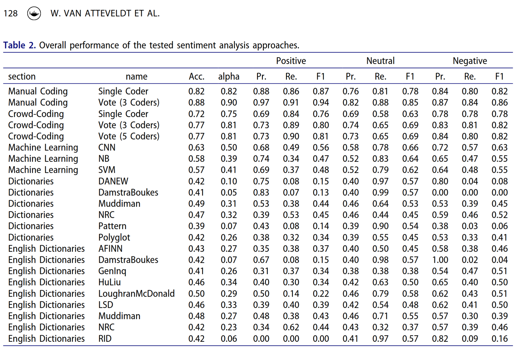
Example: Sentiment Analysis

  • gLLMs often perform better on standard text classification problems
  • Let’s put this to a test with data from Atteveldt, Velden, and and (2021)
  • What do they do? Compare trained human annotators, crowd-coding, dictionary approaches, and supervised machine learning algorithms (including deep learning) on Dutch sentiment

The Setup

Get the data

sentiment_data <- "https://raw.githubusercontent.com/vanatteveldt/ecosent/master/data/intermediate/sentences_ml.csv" |>
  read.csv() |>
  dplyr::filter(gold)

define queries and an output schema.

queries_list <- make_query(
  text = sentiment_data$headline,
  prompt = "Annotate the sentiment in this text"
)

output_schema <- list(
  "object",
  properties = list(
    sentiment = list(
      type = "string",
      enum = c("negative", "neutral", "positive")
    )
  ),
  required = "sentiment"
)
  • Using the structured output, we can make sure it is easy to process the results.

Testing the setup

query(
  queries_list[1],
  model = "llama3.2:3b-instruct-q8_0",
  screen = FALSE, # turn off priting answers
  model_params = list(seed = 42),
  output = "text",
  format = output_schema
) |>
  purrr::map(jsonlite::fromJSON) |>
  purrr::map_chr("sentiment")
[1] "positive"

Comparing a few models

extract_sentiment <- function(resp) {
  saveRDS(resp, "resp.rds")
  resp |>
    purrr::map_chr(c("message", "content")) |>
    purrr::map(jsonlite::fromJSON) |>
    purrr::map_chr("sentiment", .default = "")
}

extract_time <- function(resp) {
  purrr::map_dbl(resp, "eval_duration") * 1e-9
}

pb <- list(
  format = c("{cli::pb_spin} {cli::pb_percent} done [ETA: {cli::pb_eta}]")
)

bench_file <- "data/sentiment_bench.rds"
if (file.exists(bench_file)) {
  bench <- readRDS(bench_file)
} else {
  bench <- sentiment_data |>
    tidyr::expand_grid(
      model = c(
        "llama2:7b",
        "llama3:8b",
        "llama3.1:8b",
        "llama3.2:3b",
        "llama3.2:3b-instruct-q8_0",
        "llama3.3:70b",
        "llama3.1:70b-instruct-q5_1",
        "deepseek-r1:7b",
        "deepseek-r1:8b",
        "deepseek-r1:14b",
        "qwen2.5:7b",
        "gemma:2b",
        "gemma:7b",
        "gemma2:9b",
        "deepseek-r1:1.5b",
        "smollm2:latest",
        "qwq:32b"
      )
    ) |>
    dplyr::arrange(model) |>
    dplyr::mutate(
      query = make_query(
        text = headline,
        prompt = "Annotate the sentiment in this text"
      ),
      resp = query(
        query,
        model = model,
        screen = FALSE, # turn off printing answers
        model_params = list(seed = 42),
        output = "response",
        verbose = pb,
        format = output_schema
      ),
      sentiment = extract_sentiment(resp),
      eval_time = extract_time(resp)
    )
  saveRDS(bench, bench_file)
}

benchmark_data <- bench |>
  mutate(
    annotation_human = c("negative", "neutral", "positive")[value + 2],
    annotation_human = as.factor(annotation_human),
    sentiment = ifelse(sentiment == "", NA_character_, sentiment),
    sentiment = as.factor(sentiment)
  )

Results

model accuracy precision recall f_meas
deepseek-r1:7b 0.36 0.59 0.37 0.23
smollm2:latest 0.4 0.27 0.45 0.34
deepseek-r1:8b 0.51 0.58 0.55 0.44
deepseek-r1:14b 0.52 0.61 0.56 0.45
deepseek-r1:1.5b 0.4 0.44 0.42 0.46
llama3.2:3b-instruct-q8_0 0.51 0.5 0.51 0.49
llama2:7b 0.52 0.51 0.55 0.49
gemma:2b 0.51 0.5 0.51 0.5
llama3.2:3b 0.53 0.54 0.54 0.51
gemma:7b 0.57 0.64 0.6 0.54
llama3:8b 0.59 0.58 0.61 0.57
llama3.1:8b 0.63 0.64 0.62 0.63
qwen2.5:7b 0.64 0.67 0.63 0.64
gemma2:9b 0.68 0.71 0.71 0.67
qwq:32b 0.7 0.72 0.7 0.71
llama3.3:70b 0.72 0.72 0.73 0.73
Table 1: Performance of the tested models for sentiment analysis on data from Atteveldt, Velden, and and (2021)

Example: Improved machine learning

  • We saw earlier that these models can produce embeddings for full texts
  • These texts are dense representations of the “meaning” of text
  • We can use them to improve supervised machine learning approaches

The Setup

Get the data

set.seed(1)
reviews <- readRDS("data/imdb.rds") # |>
  # sample to make this quicker
  # slice_sample(n = 5000)

Turn them into embeddings

reviews_embeddings <- reviews |>
  mutate(embeddings = embed_text(text = text, model = "nomic-embed-text")) |>
  select(id, label, embeddings) |>
  unnest_wider(embeddings)
reviews_embeddings |> 
  select(1:10)
# A tibble: 50,000 × 10
      id label    dim_1  dim_2 dim_3   dim_4   dim_5 dim_6   dim_7  dim_8
   <int> <fct>    <dbl>  <dbl> <dbl>   <dbl>   <dbl> <dbl>   <dbl>  <dbl>
 1     1 neg    0.00258 -0.171 -2.74 -0.706  -0.488   1.48 -0.479  -0.193
 2     2 neg   -0.497   -0.623 -3.53 -0.0592  0.424   1.17 -0.839  -0.249
 3     3 neg    0.230   -0.531 -2.39  0.0430 -0.616   1.64 -0.209   0.957
 4     4 neg    0.102    0.309 -2.26 -0.373   0.850   1.30  0.595   0.366
 5     5 neg   -0.312   -0.246 -2.78 -0.237   0.226   1.31  0.303   0.644
 6     6 neg    0.146    0.375 -2.91  0.935   1.28    1.23  0.237   0.529
 7     7 neg    0.289    0.275 -3.25  0.692   0.216   1.30  0.307   1.57 
 8     8 neg   -0.0703   0.513 -3.46  1.21    0.0697  1.43  0.0469  1.26 
 9     9 neg    0.522    0.421 -2.90 -0.149  -0.760   1.58 -0.0315 -0.630
10    10 neg    0.853   -0.428 -2.90 -0.312   0.367   1.35 -1.13    0.755
# ℹ 49,990 more rows

Use tidymodels

library(tidymodels)
# split data into training an test set (for validation)
set.seed(1)
reviews_split <- initial_split(reviews_embeddings)

reviews_train <- training(reviews_split)

# set up the model we want to use
lasso_spec <- logistic_reg(penalty = tune(), mixture = 1) |>
  set_engine("glmnet")

# we specify that we want to do some hyperparameter tuning and bootstrapping
param_grid <- grid_regular(penalty(), levels = 50)
reviews_boot <- bootstraps(reviews_train, times = 10)

# and we define the model. Here we use the embeddings to predict the rating
rec_spec <- recipe(label ~ ., data = select(reviews_train, -id))

# bringing this together in a workflow
wf_fh <- workflow() |>
  add_recipe(rec_spec) |>
  add_model(lasso_spec)

# now we do the tuning
set.seed(42)
lasso_grid <- tune_grid(
  wf_fh,
  resamples = reviews_boot,
  grid = param_grid
)

# select the best model
wf_fh_final <- wf_fh |>
  finalize_workflow(parameters = select_best(lasso_grid, metric = "roc_auc"))

# and train a new model + predict the classes for the test set
final_res <- last_fit(wf_fh_final, reviews_split)

# we extract these predictions
final_pred <- final_res |>
  collect_predictions()

Check out results

library(gt)
my_metrics <- metric_set(accuracy, kap, precision, recall, f_meas)

my_metrics(final_pred, truth = label, estimate = .pred_class) |> 
  # I use gt to make the table look a bit nicer, but it's optional
  gt() |> 
  data_color(
    columns = .estimate,
    fn = scales::col_numeric(
      palette = c("red", "orange", "green"),
      domain = c(0, 1)
    )
  )
.metric .estimator .estimate
accuracy binary 0.9264800
kap binary 0.8529560
precision binary 0.9239043
recall binary 0.9282258
f_meas binary 0.9260600

Comparison to day-3: F1 = 0.72 and 0.71

Conclusion

Conclusion

  • LLMs bring many new possibilities for new research
  • A lot of it is untested and comes with risks
  • If you want to use models, think about: responsibility
  • Trust but verify!

References

Atteveldt, Wouter van, Mariken A. C. G. van der Velden, and Mark Boukes and. 2021. “The Validity of Sentiment Analysis: Comparing Manual Annotation, Crowd-Coding, Dictionary Approaches, and Machine Learning Algorithms.” Communication Methods and Measures 15 (2): 121–40. https://doi.org/10.1080/19312458.2020.1869198.
Bender, Emily M., Timnit Gebru, Angelina McMillan-Major, and Shmargaret Shmitchell. 2021. “On the Dangers of Stochastic Parrots: Can Language Models Be Too Big? 🦜.” In Proceedings of the 2021 ACM Conference on Fairness, Accountability, and Transparency, 610–23. Virtual Event Canada: ACM. https://doi.org/10.1145/3442188.3445922.
Frankfurt, Harry G. 2005. On Bullshit. Princeton, NJ: Princeton University Press. https://doi.org/10.1515/9781400826537.
Gilardi, Fabrizio, Meysam Alizadeh, and Maël Kubli. 2023. “ChatGPT Outperforms Crowd Workers for Text-Annotation Tasks.” Proceedings of the National Academy of Sciences 120 (30). https://doi.org/10.1073/pnas.2305016120.
Grimmer, J., and B. M. Stewart. 2013. “Text as Data: The Promise and Pitfalls of Automatic Content Analysis Methods for Political Texts.” Political Analysis 21 (3): 267–97. https://doi.org/10.1093/pan/mps028.
Heseltine, Michael, and Bernhard Clemm von Hohenberg. 2023. “Large Language Models as a Substitute for Human Experts in Annotating Political Text.” OSF. https://doi.org/10.31219/osf.io/cx752.
Hicks, Michael Townsen, James Humphries, and Joe Slater. 2024. ChatGPT Is Bullshit.” Ethics and Information Technology 26 (2): 38. https://doi.org/10.1007/s10676-024-09775-5.
Törnberg, Petter. 2023. “ChatGPT-4 Outperforms Experts and Crowd Workers in Annotating Political Twitter Messages with Zero-Shot Learning.” arXiv. http://arxiv.org/abs/2304.06588.
Vaswani, Ashish, Noam Shazeer, Niki Parmar, Jakob Uszkoreit, Llion Jones, Aidan N. Gomez, Lukasz Kaiser, and Illia Polosukhin. 2017. “Attention Is All You Need.” arXiv. https://doi.org/10.48550/ARXIV.1706.03762.
Weber, Maximilian, and Merle Reichardt. 2023. “Evaluation Is All You Need. Prompting Generative Large Language Models for Annotation Tasks in the Social Sciences. A Primer Using Open Models.” https://arxiv.org/abs/2401.00284.
Zhong, Qihuang, Liang Ding, Juhua Liu, Bo Du, and Dacheng Tao. 2023. “Can ChatGPT Understand Too? A Comparative Study on ChatGPT and Fine-Tuned BERT.” arXiv. http://arxiv.org/abs/2302.10198.

Footnotes

  1. but still need of validation!