Computational Text Analysis
Module 03 GESIS Fall Seminar “Introduction to Computational Social Science”
text-as-data methods
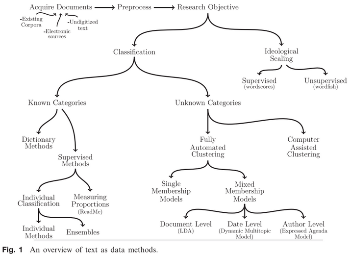
From Grimmer and Stewart (2013)
text-as-data methods
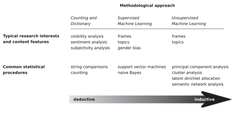
From Boumans and Trilling (2015)
text-as-data methods
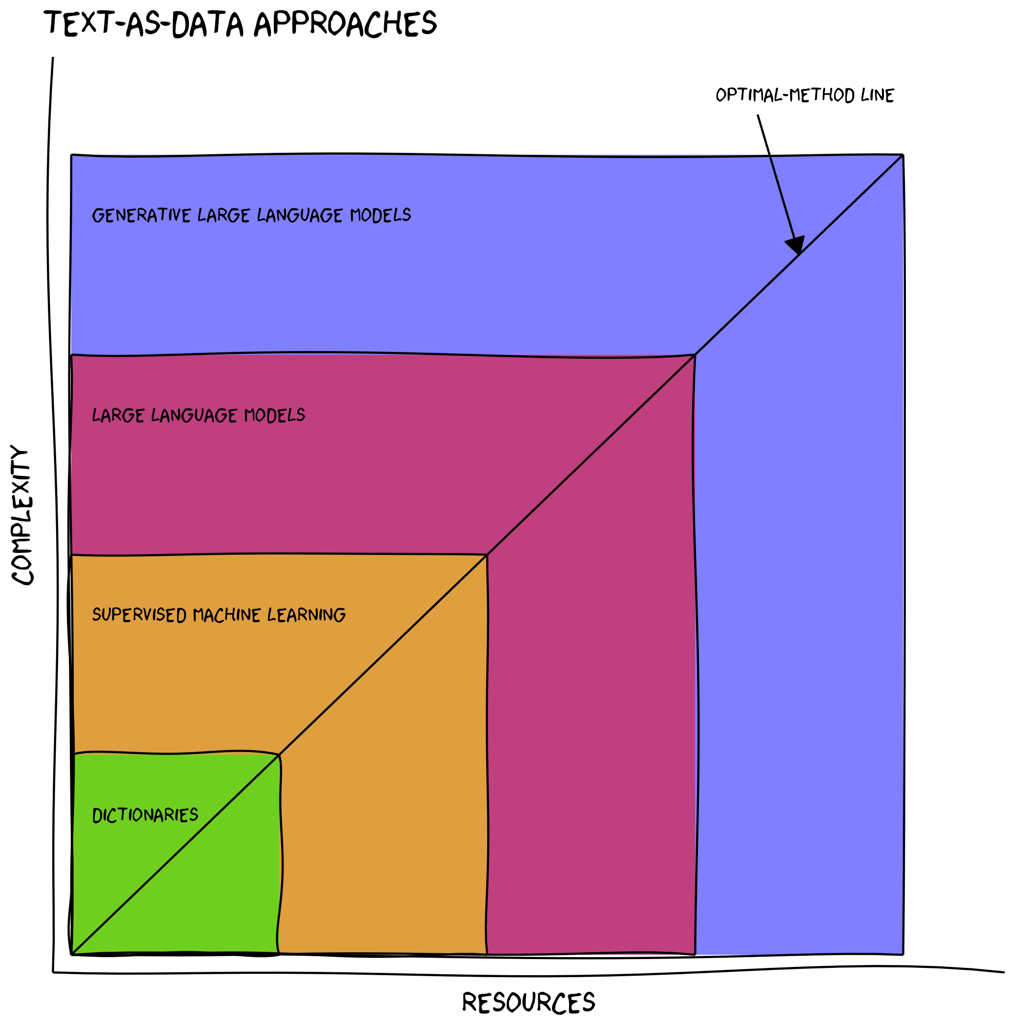
From myself.
What are Dictionary-based Approaches?
- Lexicon/Dictionary: the words in a language and their meaning
- Lexicon/Dictionary-based approaches: simply count how often pre-defined words appear to infer meaning of text
- Wordcounts are usualy used to categorise text (e.g., non-/relevant, positive/negative, a-/political)
- To infer category from count, researchers define mapping function (e.g., N positive terms > N negative terms = positive text)
- Like ‘normal’ dictionaries: several forms of the word carry same meaning, expressed through wildcards (e.g., econom*) or regular expressions (e.g., econom.+) (matches economists, economic, and so on)

Example: Non-Consupmtive Research with Google Books
Taken from Duneier (2017): Ghetto: The Invention of a Place, the History of an Idea
- RQ: How did the meaning of ghetto change over time?
- Method: Non-Consumptive Research with the Google Books Ngram Viewer
# Ngram data table
# Phrases:
# Case-sensitive:
# Corpuses:
# Smoothing:
# Years: 1920-1975
Year Phrase Frequency Corpus Parent type
1 1920 ghetto 5.954661e-08 en NGRAM
2 1921 ghetto 4.997540e-08 en NGRAM
3 1922 ghetto 6.947938e-08 en NGRAM
4 1923 ghetto 7.295493e-08 en NGRAM
5 1924 ghetto 7.934730e-08 en NGRAM
6 1925 ghetto 2.008454e-07 en NGRAMggplot(ng, aes(x = Year, y = pct, colour = Phrase)) +
geom_line() +
theme(legend.position = "bottom")
Plotting the scores
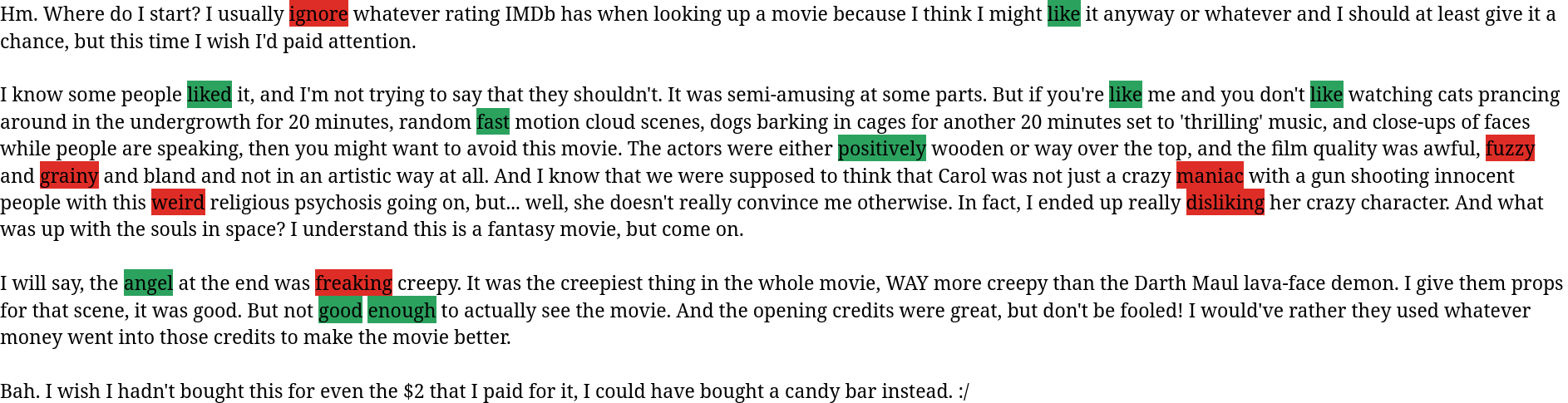
We can plot these results to get an impression how often each category was predicted and how strong the senti_score was in these cases.

Issues
- The more terms we add to our dictionary, the more false positives we will get
- Building a good dictionary is a lot of work (complexity-resource plot):
- Negation and bag-of-word issues (“not good” will be counted as positive + modifiers such as “very good”)
- “great” should be more positive than “good”
- Negative image of dictionaries in academia
- Many negative examples where dictionaries were applied often outside of the domain they had been developed
- Wrong believe that popular off-the-shelf dictionaries do not need validation
- Many papers that show that dictionaries do not perform as well as machine learning: e.g. Van Atteveldt, Van Der Velden, and Boukes (2021); González-Bailón and Paltoglou (2015); Boukes et al. (2020)
Now that you know about dictionaries, remember to apply them only under some circumstances:
- When no other method is available, e.g., in data retrieval or nonconsumptive research
- Variable we want to code is manifest and concrete rather than latent and abstract: names of actors, specific physical objects, specific phrases, etc., rather than feelings, frames, or topics.
- All synonyms to be included must be known beforehand.
- And third, the dictionary entries must not have multiple meanings.
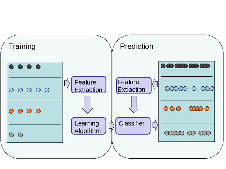
What are Supervised Machine Learning Approaches?
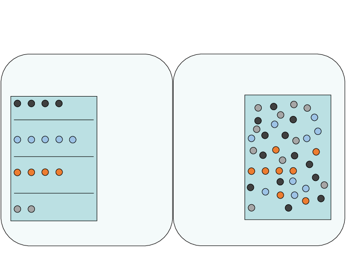
What are Supervised Machine Learning Approaches?
What should you use?
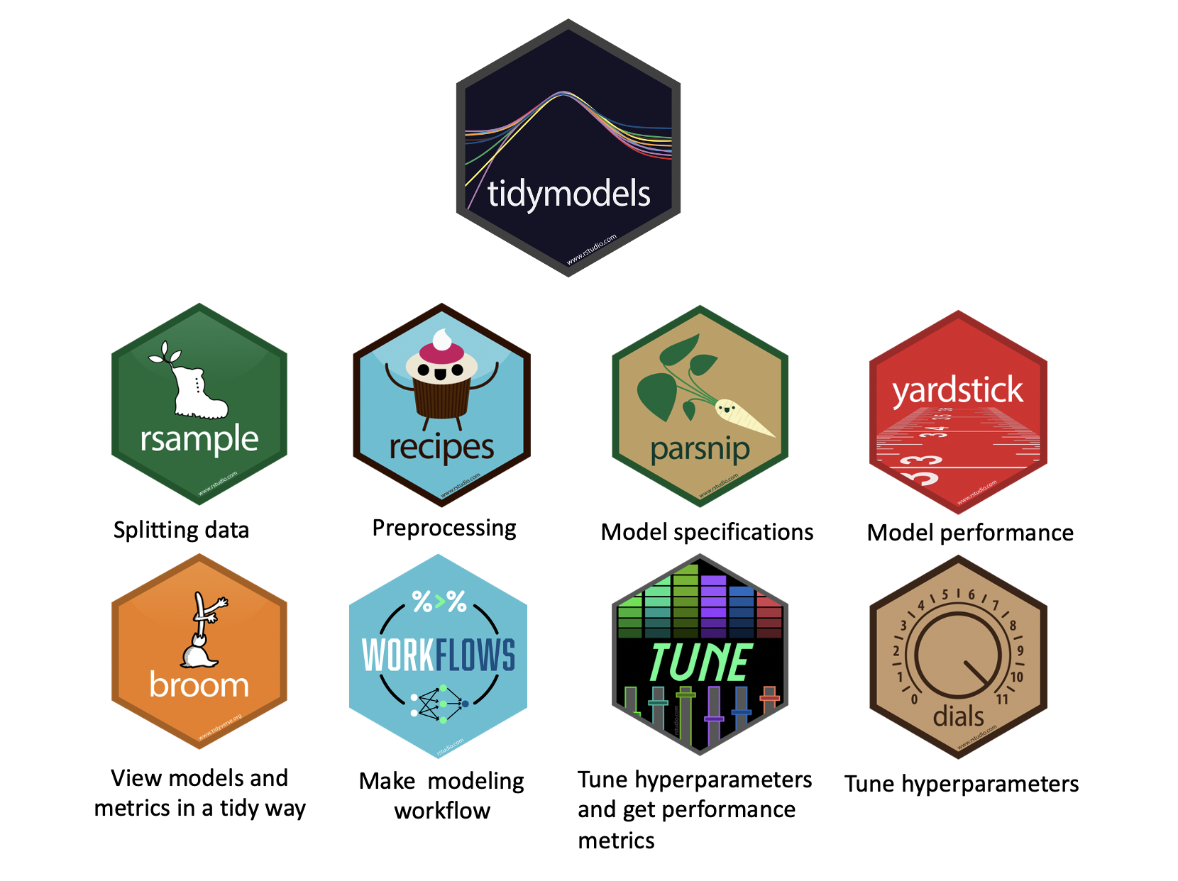
Several frameworks in R:
RTextTools: includes the most important algorithms, but outdatedcaret: includes a huge variety of models and comes with robust helper functions, but supersededquanteda: nice suite of text analysis functions, includingquanteda.textmodelstidymodels: successor ofcaretwith an extensive collection of algorithms, preprocessing, validation and comparison functions
Additional step: looking inside the model
A way to make sense of a model is to look at coefficients. This tells us essentially, what the model thinks are important terms to say a document is positive or negative.
model_lasso |>
extract_fit_engine() |>
vip::vi() |>
group_by(Sign) |>
slice_max(Importance, n = 20) |>
ungroup() |>
mutate(
Variable = str_remove(Variable, "tf_text_"),
Variable = fct_reorder(Variable, Importance)
) |>
ggplot(aes(x = Importance, y = Variable, fill = Sign)) +
geom_col(show.legend = FALSE) +
facet_wrap(~Sign, scales = "free_y") +
labs(y = NULL)
Learn more
- Emil Hvitfeldt, Julia Silge: Supervised Machine Learning for Text Analysis in R, https://smltar.com/

Playful exploration1
A good first step towards understanding what topic models are and how they can be useful, is to simply play around with them, so that’s what we’ll do first. Open the page https://lettier.com/projects/lda-topic-modeling/ (if possible, in Firefox)
Example Docs:
- 🐭 🐭 🐭 🐭 🐭 🐭 🐭 🐭 🐭 🐭
- 🐱 🐱 🐱 🐱 🐱 🐱 🐱 🐱 🐱 🐱
- 🐶 🐶 🐶 🐶 🐶 🐶 🐶 🐶 🐶 🐶
- 🐭 🐭 🐭 🐭 🐭 🐭 🐭 🐭 🐭 🐭 🐱 🐱 🐱 🐱 🐱 🐱 🐱 🐱 🐱 🐱 🐶 🐶 🐶 🐶 🐶 🐶 🐶 🐶 🐶 🐶
On top, the texts are turned into a document feature matrix.
Playful exploration
The first matrix describes the probability a feature belongs to a topic. We call this the feature-topic-matrix:
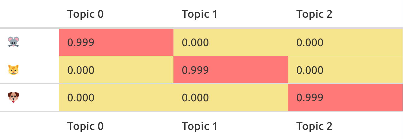
This case makes it pretty clear:
- mice belong into the first topic
- cats belong into the second
- dogs belong into the third topic
Playful exploration
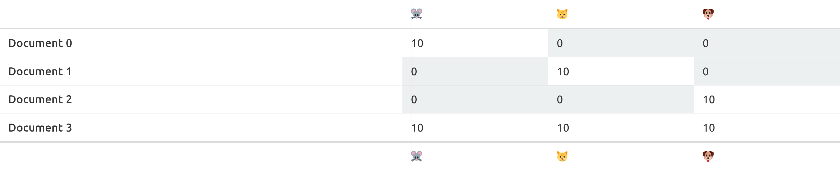
The second table does the same, but with documents. We call this the document-term-matrix:
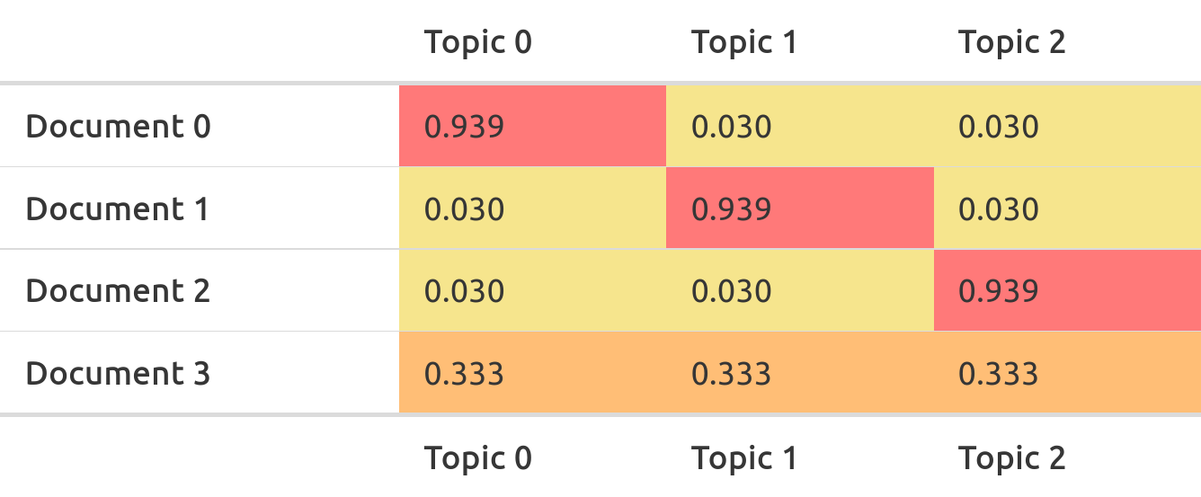
- The first document has a high probability to belong to the first topic, because it is full of mice
- The second document has a high probability to belong to the second topic, because it is full of cats
- The third document has a high probability to belong to the third topic, because it is full of dogs
(3) Inspecting and analysing the results
Word-topic probabilities
bundestag18_ftm <- lda_model$phi |>
as.data.frame() |># converting the matrix into a data.frame makes sure it plays nicely with the tidyverse
rownames_to_column("topic") |># the topic names/numbers are stored in the row.names, I move them to a column
mutate(topic = fct_inorder(topic)) |># turn to factor to maintain the correct order
pivot_longer(-topic, names_to = "word", values_to = "phi")
topic_topwords_plot <- bundestag18_ftm |># turn to long for plotting
group_by(topic) |># using group_by and slice_max, we keep only the top 10 values from each topic
slice_max(order_by = phi, n = 15) |>
# using reorder_within does some magic for a nicer plot
mutate(word = tidytext::reorder_within(word, by = phi, within = topic)) |>
# from here on, we just make a bar plot with facets
ggplot(aes(x = phi, y = word, fill = topic)) +
geom_col() +
tidytext::scale_y_reordered() +
facet_wrap(~topic, ncol = 2, scales = "free_y")
topic_topwords_plot
Going forward, I would now name these topics. I found this particular format in a Excel sheet helpful.
lda_model$phi |>
as.data.frame() |>
rowid_to_column("topic") |>
pivot_longer(-topic, names_to = "word", values_to = "phi") |>
group_by(topic) |>
slice_max(order_by = phi, n = 20) |>
mutate(top = row_number()) |>
pivot_wider(id_cols = top, names_from = topic, values_from = word) |>
# Add an extra row where you can write in topic names
add_row(top = NA, .before = 1) %>%
rio::export("topicsmodel_topwords.xlsx")Topics per document
Similarly to above, we can also extract to topics per document:
bundestag18_dtm <- lda_model$theta |>
as.data.frame() |>
rownames_to_column("doc_id") |>
as_tibble()
bundestag18_dtm# A tibble: 51,798 × 11
doc_id topic1 topic2 topic3 topic4 topic5 topic6 topic7 topic8 topic9 topic10
<chr> <dbl> <dbl> <dbl> <dbl> <dbl> <dbl> <dbl> <dbl> <dbl> <dbl>
1 2013-… 0.0936 0.171 0.355 0.0195 0.0890 0.0667 0.0371 0.0306 0.103 0.0343
2 2013-… 0.260 0.0632 0.123 0.0421 0.0632 0.0246 0.0772 0.214 0.0421 0.0912
3 2013-… 0.0980 0.0980 0.0980 0.0980 0.0980 0.118 0.0980 0.0980 0.0980 0.0980
4 2013-… 0.112 0.0875 0.112 0.075 0.075 0.0625 0.138 0.15 0.1 0.0875
5 2013-… 0.0909 0.0909 0.109 0.0909 0.0909 0.127 0.0909 0.0909 0.0909 0.127
6 2013-… 0.255 0.0691 0.112 0.0372 0.0638 0.0426 0.122 0.0904 0.0585 0.149
7 2013-… 0.0943 0.0943 0.0943 0.0943 0.0943 0.113 0.0943 0.0943 0.0943 0.132
8 2013-… 0.257 0.0616 0.0978 0.0290 0.0435 0.0399 0.0833 0.207 0.0652 0.116
9 2013-… 0.0865 0.0602 0.0564 0.0263 0.0338 0.0677 0.0526 0.113 0.0376 0.466
10 2013-… 0.0841 0.0561 0.0748 0.0654 0.0841 0.0841 0.0841 0.112 0.0841 0.271
# ℹ 51,788 more rowsWe can tidy this and join the results back with the original metadata using the doc_id:
bundestag18_dtm_tidy <- bundestag18_dtm |>
pivot_longer(-doc_id, names_to = "topic", values_to = "theta") |>
# again this is to keep track of the order as it is otherwise order by alphabet
mutate(topic = fct_inorder(topic)) |>
left_join(bundestag18 |> select(-text), by = "doc_id")
bundestag18_dtm_tidy# A tibble: 517,980 × 13
doc_id topic theta date agenda speechnumber speaker party
<chr> <fct> <dbl> <date> <chr> <int> <chr> <chr>
1 2013-10-22-1 topic1 0.0936 2013-10-22 SITZUNGSBE… 1 Heinz … <NA>
2 2013-10-22-1 topic2 0.171 2013-10-22 SITZUNGSBE… 1 Heinz … <NA>
3 2013-10-22-1 topic3 0.355 2013-10-22 SITZUNGSBE… 1 Heinz … <NA>
4 2013-10-22-1 topic4 0.0195 2013-10-22 SITZUNGSBE… 1 Heinz … <NA>
5 2013-10-22-1 topic5 0.0890 2013-10-22 SITZUNGSBE… 1 Heinz … <NA>
6 2013-10-22-1 topic6 0.0667 2013-10-22 SITZUNGSBE… 1 Heinz … <NA>
7 2013-10-22-1 topic7 0.0371 2013-10-22 SITZUNGSBE… 1 Heinz … <NA>
8 2013-10-22-1 topic8 0.0306 2013-10-22 SITZUNGSBE… 1 Heinz … <NA>
9 2013-10-22-1 topic9 0.103 2013-10-22 SITZUNGSBE… 1 Heinz … <NA>
10 2013-10-22-1 topic10 0.0343 2013-10-22 SITZUNGSBE… 1 Heinz … <NA>
# ℹ 517,970 more rows
# ℹ 5 more variables: party.facts.id <dbl>, chair <lgl>, terms <dbl>,
# parliament <chr>, iso3country <chr>Now, we can e.g. compare topic usage per party:
bundestag18_dtm_tidy |>
filter(!is.na(party),
party != "independent") |>
group_by(party, topic) |>
summarize(theta = mean(theta)) %>%
ggplot(aes(x = theta, y = topic, fill = party)) +
geom_col(position = "dodge") +
scale_fill_manual(values = c(
"PDS/LINKE" = "#BD3075",
"SPD" = "#D71F1D",
"GRUENE" = "#78BC1B",
"CDU/CSU" = "#121212",
"FDP" = "#FFCC00",
"AfD" = "#4176C2"
))
Or over time:


Finding an optimal number of topics
- The best way to find the optimal \(k\) number of topics is to interpret different models and look for the ones that seems to divide your corpus into the most meaningful topics
- That is very cumbersome though and there are some statistical methods to make the process easier
- The idea behind all of them is to compare the metrics of different models to narrow your search down
library(furrr)
lda_models <- "data/lda_models.rds"
# since this takes a long time, I save the results in case I want to run it again
if (!file.exists(lda_models)) {
plan(multisession) ## for parallel processing
lda_fun <- function(k, max_iter = 200) {
textmodel_lda(
bundestag18_dfm,
k = k,
max_iter = max_iter,
alpha = 50 / k,
beta = 0.1,
verbose = TRUE
)
}
models_df <- tibble(
k = c(10:20),
model = future_map(k, lda_fun, .options = furrr_options(seed = 1))
)
saveRDS(models_df, lda_models)
} else {
models_df <- readRDS(lda_models)
}There is no official function in seededlda to evaluate different models. The stm package is much better here as demonstrated by Julia Silge. But since I did not want to introduce another package, I copied the functions that are currently discussed from this issue on GitHub.
semantic_coherence <- function(model, top_n = 10) {
h <- apply(terms(model, top_n), 2, function(y) {
d <- model$data[,y]
e <- Matrix::Matrix(docfreq(d), nrow = nfeat(d), ncol = nfeat(d))
f <- fcm(d, count = "boolean") + 1
g <- Matrix::band(log(f / e), 1, ncol(f))
sum(g)
})
sum(h)
}
divergence <- function(model) {
div <- proxyC::dist(model$phi, method = "kullback")
diag(div) <- NA
mean(as.matrix(div), na.rm = TRUE)
}
# this one is taken from stm https://github.com/bstewart/stm/blob/master/R/exclusivity.R
exclusivity <- function(model, top_n = 10, frexw = 0.7) {
tphi <- t(exp(model$phi))
s <- rowSums(tphi)
mat <- tphi / s # normed by columns of beta now.
ex <- apply(mat, 2, rank) / nrow(mat)
fr <- apply(tphi, 2, rank) / nrow(mat)
frex <- 1 / (frexw / ex + (1 - frexw) / fr)
index <- apply(tphi, 2, order, decreasing = TRUE)[1:top_n, ]
out <- vector(length = ncol(tphi))
for (i in seq_len(ncol(frex))) {
out[i] <- sum(frex[index[, i], i])
}
return(mean(out))
}We can now use this plot to evaluate the different models.
models_df_metrics <- models_df |>
mutate(semantic_coherence = map_dbl(model, semantic_coherence),
exclusivity = map_dbl(model, exclusivity),
divergence = map_dbl(model, divergence))
models_df_metrics |>
select(-model) |>
pivot_longer(-k, names_to = "metric") |>
ggplot(aes(x = k, value, color = metric)) +
geom_line(linewidth = 1.5, alpha = 0.7, show.legend = FALSE) +
scale_x_continuous(breaks = scales::pretty_breaks()) +
facet_wrap(~metric, scales = "free_y") +
labs(x = "K (number of topics)",
y = NULL,
title = "Model diagnostics by number of topics",
subtitle = "Higher = Better")
Learn more
- Wouter van Atteveldt, Damian Trilling & Carlos Arcila: Computational Analysis of Communication, https://cssbook.net/

Footnotes
heavily influenced by this piece: https://medium.com/@lettier/how-does-lda-work-ill-explain-using-emoji-108abf40fa7d
